

Building a Capsule Net in Excel
Capsule networks are possibly the biggest advance in neural network design in the last decade. They appear to mimic the human brain far more than convolutional neural networks and move us significantly closer to artificial general intelligence. As a step towards demystifying these new algorithms I’ve built one on-sheet in Excel.
Fig: These GIFs stride back and forth over all 8 dimensions of the linear manifold of various digits while holding the other dimensions constant. They are from a Capsule Net built on-sheet in Excel which learns the linear manifold of the 10 MNIST handwritten digits and then uses these for categorisation of new Digits.
Since a turning point in 2012, neural networks, have become dominant in the field of machine learning and Artificial intelligence (AI). They are so named because they loosely model the structure of neurons in the brain. Nowadays, they pretty much form the default approach for computer vision, translation, speech recognition etc. Convolutional Neural Networks (ConvNets), are a sub-class of
CapsNets appear to behave more like the brain than ConvNets. Their inventor Geoff Hinton talks about these characteristics in this presentation https://youtu.be/rTawFwUvnLE , given shortly after he released the paper in late 2017. Mimicking the human brain is a promising route to our understanding and developing a theory of intelligence. An analogy is the development of a theory of aerodynamics by initially studying birds. The current fruits of this initial approach are aircraft that can circle the earth in 6 hours or carry 500 passengers across the Atlantic. With a similar trajectory, we can only wonder what a theory of intelligence will yield.
Over the last two years I’ve been trying to master and implement Neural Nets in my work. To help me get up to speed, I’ve been building in Microsoft Excel. This is slow but gives me a different and intuitive way to see how they work, and given that some of these neural networks were considered almost magical and certainly state-of-the-art quite recently, to build in Excel is quite demystifying. I’ve built several relatively large neural Networks and posted quite a few online. This batch run ConvNet with Adam optimization hits recent benchmarks for recognizing human handwriting https://youtu.be/OP7wi2MoSeM and should give you a flavour.
CapsNets are exciting and look to me like a massive development in AI that brings us closer to understanding how the human brain works or at least some of the key maths that play a part in human learning and intelligence. I say this because they learn, fail and succeed in far more human ways than do ConvNets.
- Visual twists, shifts, squeezes and expansions of objects (affine transforms) put a CapsNet off the scent far less than a ConvNet. Think of those verification “captchas” that websites present you with to prove you’re human. We are far better at recognizing distorted digit captures than ConvNets. For a ConvNet to do the same it would have had to be trained on some similar distortion before whereas a CapsNet can extrapolate along those transformations more easily. This also makes them far better at recognizing 3D objects from different viewpoints than ConvNets.
- Humans learn patterns that represent canonical objects with very few examples or rather instructions. You don’t need to subject a child to 60,000 examples of handwritten digits before they know the numbers 0 to 9. CapsNets have been trained with as few as 25 interventions. We still need to show them a load of handwritten characters but not actually tell them what these are. The advantages they offer for unsupervised learning are already phenomenal.
- CapsNets effectively take bets on what they are seeing and seek information to confirm this. This is what the core routing by agreement algorithm does. As proof builds up they instantaneously prune densely connected layers to sparsely connected layers linking lower level features to specific higher-level features. This is analogous to our making an assumption on what we see, imposing a reference frame and seeking information to fill in the rest. This only becomes apparent when we get it wrong as we generally do with trick images like this shadow face: https://www.youtube.com/watch?v=sKa0eaKsdA0
- CapsNets suffer from the human visual problem known as crowding. This is where too many examples of the same object occur closely together and simply confuse our mind, an example being – how hard it is to count the separate lines here IIIIIIII- I can’t do this as easily as reading the word seven ????.
CapsNets are effectively a vectorized version of ConvNets. In ConvNets, each neuron in a layer gives the probability of the presence of a feature defined by its kernel. CapsNets do more, they convey not only the presence but the “pose” of the feature. By
This blog post is about building a full capsule net in Excel for handwritten digit classification using MNIST data. MNIST is a data set of hand written digits provided by Yann LeCun and a staple in data science. Given the novelty of this new algorithm there is not so much information available on the net but the best I came across was Geoff Hinton’s original paper https://arxiv.org/pdf/1710.09829v2.pdf and Aurélien Géron’s Keras code and associated videos https://youtu.be/pPN8d0E3900 . I also found this talk by Dr Charles Martin helpful https://youtu.be/YqazfBLLV4U .
——- The remainder of this blog post
CapsNets are exciting and potentially far more powerful than standard convolutional neural nets because:
- They don’t lose information via subsampling or max pooling which is the ConvNet way to introduce some invariance, CapsNets weights encode viewpoint-invariant knowledge and are equivariant.
- Through the above approach, they know the “pose” of parts and the whole which allows them to extrapolate their understanding of geometric relationships to radically new viewpoints (equivariance),
- They have built-in knowledge of the relationship of parts to a whole.
- They contain the notion of entities and those GIFs on the top of the blog represent movement along one dimension of the linear manifold of the top level entity that represents an eight.
The Hinton & Géron resources were superb for the forward model i.e. the algorithm that identifies categories based on trained parameters which
How a capsule net works
I’ve uploaded a video walkthrough of the Excel model here: https://youtu.be/4uiFJZjw6fU It’s probably not for the casual reader but is a more visual way to see what’s happening and also covers a lot of the issues I’ve written about in this blog.
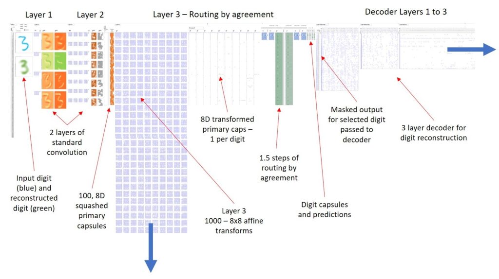
A big difference between CapsNets and standard neural networks is that CapsNets contain the notion of entities with pose parameters i.e. the network identifies component parts (lower level capsules) and determines if their pose parameters match those of the higher-level capsules where these parts are combined. Capsules require multiple dimensions to convey their pose and the diagram below shows where the additional dimensions appear:
FThe CapsNet I built is like the structure in
Hinton’s paper but quite a bit smaller with 5×5 kernels for 4 & 8 channels
in the first two layers and 8-dimensional Digit Capsules. This gives only 100 x
8D primary capsules and 10 x 8D digit capsules. The results for this are still
impressive i.e. 98.7% accuracy rather than the 99.5% accuracy that we see with
1152 x 8D primary and 10 x 16D digit capsules in the paper. I chose this
reduction after paring down the Keras model to a size that would be manageable
in Excel without too much Excel build optimization. The structure of my forward
CapsNet, or rather a screenshot of the actual CapsNet as it appears in my Excel
spreadsheet, is below.
The backpropagation or learning mechanism is much bigger. In the figure below, I’ve put together several screen-shots of the entire spreadsheet model. This covers 1000 rows and 7500 columns. The bulk of the area relates to the decoder sections with their 784 neurons in the final layer and the Adam optimization I used to get the learning speed up. I’ve highlighted the big blue collection of layer 3 transform matrices on this to give you an indication of the size w.r.t. the above forward model, additional calculations, and complexity required for the backward pass.

The Process of Building.
Now I know what I’m doing I could probably mechanically build this in a couple of days or modify the size of a layer in an hour or so. However, if I built it in Keras it would take a couple of hours and
My initial approach was to build only the forward model and feed this with pre-trained parameters from a modified version of Aurélien Géron’s code. My reduced spec (L1: 5x5K, 4c, L2: 5×5, 8c s2 L3: 8Dx10caps, Decoder 50, 50, 784) took the parameter count down from the 44,489,744 of the original paper that Aurélien had replicated to a more Excel manageable 127,943. Keras trials on this gave an MNIST test result of 98.69%, higher that I could regularly obtain with my Excel ConvNets but way below the 99.43% that the bigger model achieves.
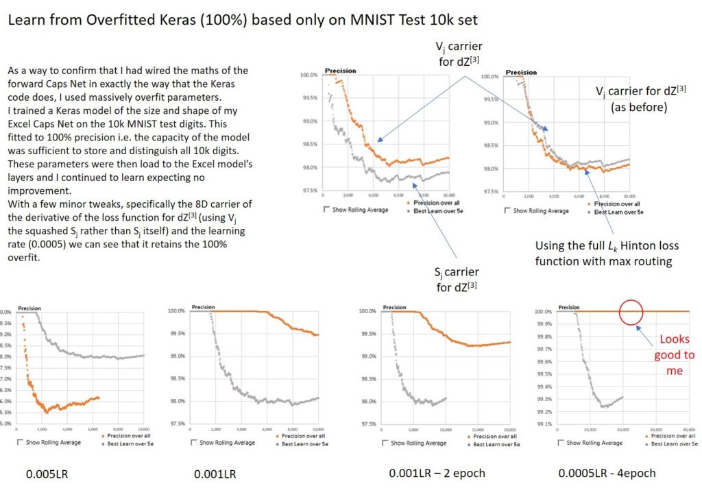
Another important modification I made to get a clear comparison was to initially train and test the reduced size Keras model only on the 10k MNIST data set. This reached a 100% overfit after about 34 epochs. What I mean by this is that the model was able to learn the 10K data set to 100% accuracy i.e. the model could store sufficient information in its parameters to categorize all 10k MNIST digits correctly. This is useless as a generalizable model but gave me an easy test to see if the Keras trained parameters, when transferred to Excel would deliver the same result on the same test set.
I was on several steep learning curves throughout this process and was delighted when I eventually got a perfect match. However, as I added the backward model and learned from these already overfit parameters, the model’s precision collapsed to 30% or so and only then began to learn. I saw more failure modes than I can recall and given the slow speed at which the excel model learned had plenty of time to hypothesize the causes.
I began this process in August of 2018 and eventually confirmed that I had a working CapsNet in Excel on 31-December 2018. The closing stages of using this odd approach of matching to a 100% overfit are summarized below.
Once I had confirmation that it was eventually working, adding the full 60k digit training data, loading 50 epoch Keras trained parameters and running a 10k test in Excel that matched the 98.69% Keras Test result took no time. I headed out happy that night to celebrate the new year.
Interesting Learning
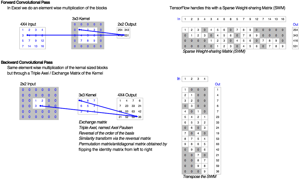
Triple Axel
One challenge that I faced was wiring the back propagation of the convolutions. Though I now know this to be straightforward, I went through the process without really thinking through the maths or approach and miraculously ended up with the right answer. On further research I found that this obscure transpose and flip of the kernel over its anti-diagonal is apparently called a Triple Axel named after a figure skater from the 19th century. This is according to User1551 on math.stackexchange, though I can’t find any other evidence, I love the idea and am happy to propagate the meme.
In TensorFlow and as I understand it,
In Excel, the Triple Axel transformation of the kernel is much easier to code, use and audit, so makes for a nice approach.
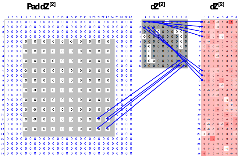
Backpropagation through a stride
I tried many attempts at getting this to work before I began looking for a proper explanation. The best I came across was “A guide to convolution arithmetic for deep learning” by Vincent Dumoulin and Francesco Visin from Institut des algorithmes d’apprentissage de Montréa. I would check their paper out if you’re confused.
Ultimately the wiring in Excel for this is very straightforward and simply requires interspersing zeros in the post-stride channel to bring the size of the channel up to the pre-stride size as shown below. The re-shaping from the 8D capsule gradients was also straightforward and the figure below shows how I unrolled these capsules into the convolutional channels. Again, I tried all sorts of approaches to this simple unfurling of the channels and arrived at the correct one by chance.
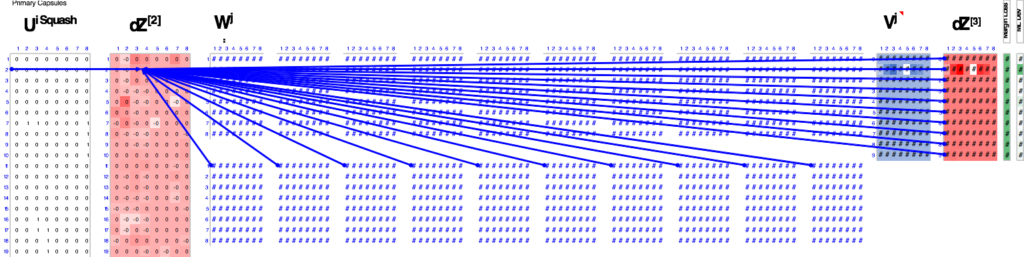
Backprop through the affine transforms
I spent some time working through ways to build the derivative of the layer 2 output function dZ[2] This comprises a sum of the matrix products of each transformation matrix by the dZ[3] and routed via the derivative of the Layer 2 activation function i.e. only pass the gradient back if the
Margin loss & “Brim Loss?”
Generating a dZ[3] with the right dimension (8D) to pass back through the affine transforms also caused me some issues. I tried various approaches but the one that mimicked TensorFlow, and one I therefore assumed to be correct, was simply to multiply the derivative of the loss function by the final digit capsule vectors i.e. after the vector nonlinearity or squash function.
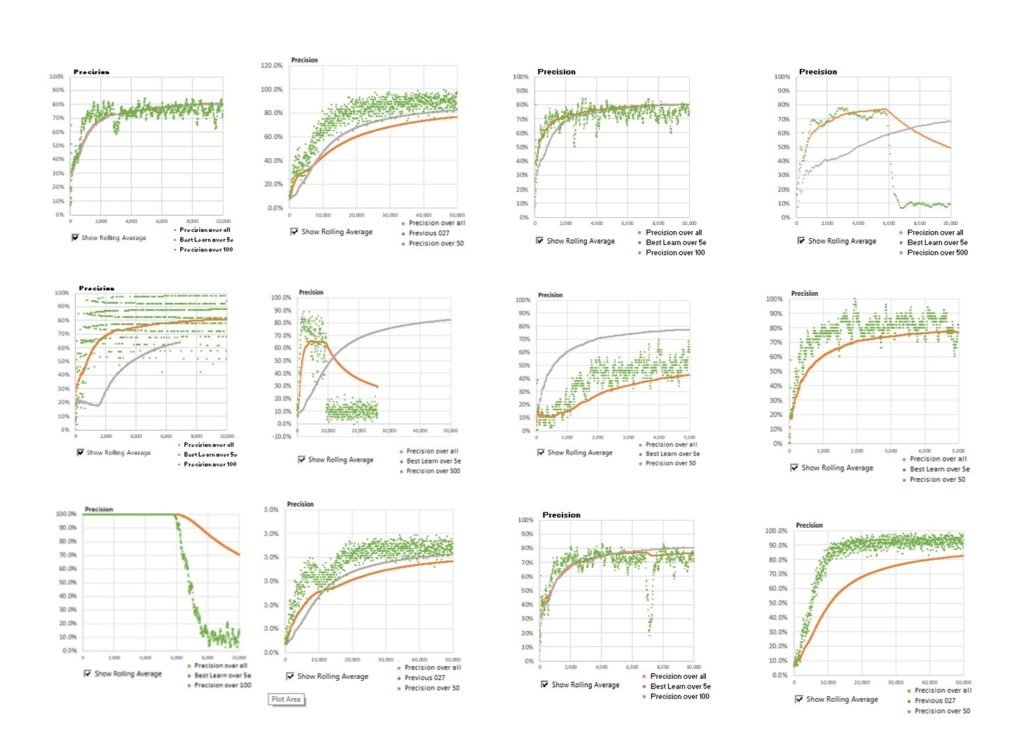
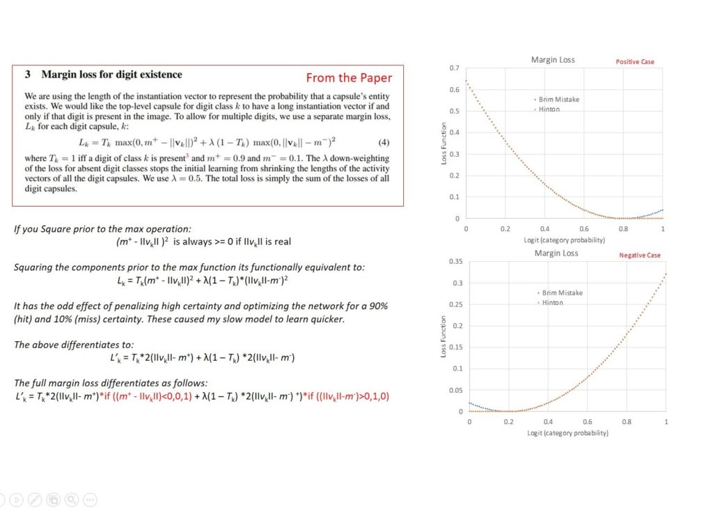
I used the margin loss quoted in the paper but made some silly mistakes in calculating its derivative that negated the use of the max function and instead of ignoring gradients for activations greater than 90% and less than 10%, actually penalized high certainty above and below the thresholds. This effectively optimized for uncertainty or specifically a 90% certainty of true and a 10% certainty of false. An interesting result of this was that the model trained up to the 100% overfit benchmark I was using faster. This approach also potentially introduces additional regularization at little cost in time and code.
Because Excel is so slow I’ve stuck with this approach and until I find the correct name for it am calling it a “Brim” loss because the resulting loss curve looks like the brim of a hat. I explain this further in the figure below.
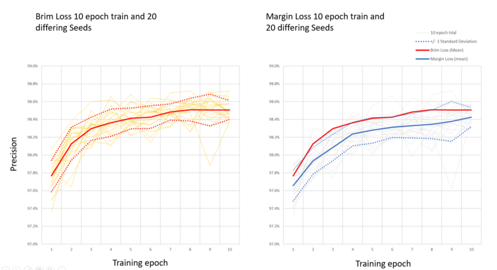
I ran 20 learning trials over 10 epochs for both the Margin Loss and the Brim loss, each with differing seeds for initialization. Multiple trials are the only way to get a rough measure of the advantage that the Brim loss may offer over the margin loss in this case. The trials below show the learning curves (as precision rather than loss) and the improvement is quite substantial. These were, of
The Next Steps
If I carry this further in Excel I think the next step will be to introduce an innate graphics model along the lines of “Extracting pose information by using a domain specific decoder” Navdeep Jaitly & Tijmen Tieleman. This will allow the model to run unsupervised learning to go from pixels to entities with poses and opens the ability to train on MNIST to with only a handful of supervised inputs.
I’m also keen to explore Matrix capsules, EM routing, running on the SmallNORB data set and of course optimizing Excel to run more quickly, perhaps making use of the iterative functions in Excel. I’ll update this blog as I make progress but would welcome any encouragement or tips and corrections.
Juergen
January 14, 2019 at 1:06 pmHi Richard,
very impressive what you are doing there! This is amazing stuff, never thought that Excel can go as far as this, but it seems that you have to have an unbelievable knowledge about this!
Thanks
Juergen
Richard Maddison
January 14, 2019 at 3:23 pmThank you, Juergen,
I’m really excited by this beast of an algorithm and am already finding uses for it in the real (Python/Tensorflow) world.
Best wishes,
Richard
Enrique Luengo
January 17, 2019 at 1:05 amGlad to see that you continue with your researching activity and happy to find that you still post with such a nice detail. Thank you Richard. Keep going.
enrique luengo
January 26, 2019 at 4:27 pmMy past intentions where to learn ANN from samples, purpose I did not achieve. Not only because it’s nearly impossible to get to the core from any sample built in a framework (as they are a black hole), either because open models are hard to find.
I was decided to change my halted advances about this subject. So I started with a full course on a MOOC (deeplearning.ai, but could also have been the fast.ai one). It’s not hard to confess that I were totally wrong from the beginning. For the newbes (as I’m), I have only this recommendation, you MUST go through one of this courses just to have a barely idea of what’s is going on. There is a lot of algebra implied (to get the thing in a nice shape), and a lot of tricks to get the shape fit (convoluting, pooling, padding, striding,…).
If you’re like me, I was so eager to learn that fully completed 3 of 5 Andrew Ng courses under a week.
So, it’s now that I’m starting to understand the graphics you post in this blog, or why are those noisy charts there.
But even I had listened to all the interviews in that course, and Geoffrey Hinton was the first one, I did not get noticed of the capsule networks until now. I imagined him as a respetable man doing his things in his lab/university and sendind papers that were not accepted… (I though, for myself. what can he share if the community is not hearing him?). Thank you for posting this.
If anyone else interested I would recommend to take a look at Max Pechyonkin posts (Hinton’s Capsule Networks Series), as I think they are a bit less academic than the papers.
I made myself a purpose to VBA/Excel a ConvNet add-in this year. It’s eleven months from now to see if I reach the target.
See ya!. And keep posting